スキップしてメイン コンテンツに移動

Visualization of Variational method

Introduction
Today, I will implement visualization of Variational method. Variational method is used when we want to minimize functional. functional is function of function. Please look at [1],[2],[3],[5] and [6].

Overview

  • formula 
  • Implementation
  • Visualization
Formula
I used following formula.
$$F(x) = \sqrt{1+(\frac{du}{dx}(x))^2}$$
$$l(u) = \int_{0}^{1} \sqrt{1+(\frac{du}{dx}(x))^2} dx$$

l(u) is the length of the u(x). 
I want to minimize l(u) subject to $u(0)=a$ and $u(1)=b$.
u minimizing I(u) is 
$$u(x) = (b-a)x+a$$

This u is line from (0,a) to (1,b).
Because l(u) is the length of the u(x), We found out that u minimizing l(u) is line.

Please look [5] to calculate of variational method.

Implementation
I implement visualization of variational method to check difference of optimize curve and other curve. 
Let $u_A$ is 
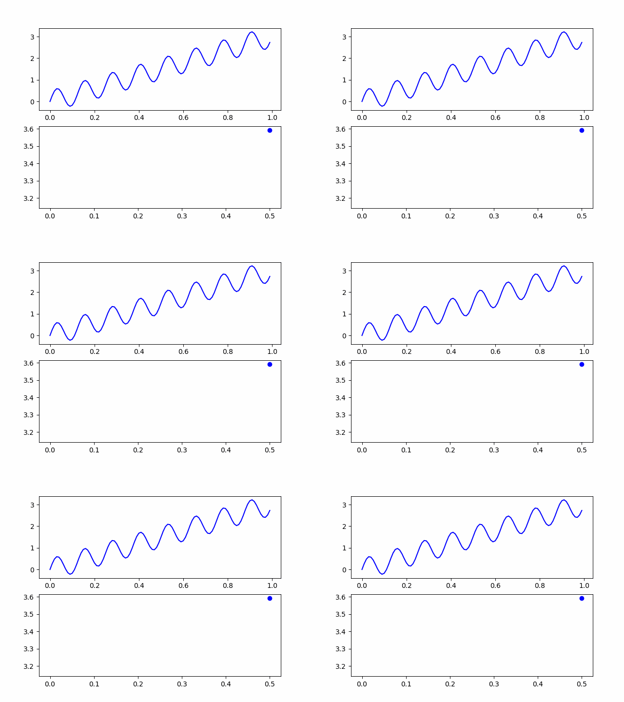
$$u_A = (b-a)x+a + A sin(8t)$$
$A sin(8t)$ increase the distance from $u$. $A \in [0,0.5]$.

If $A=0$, u is optimization curve. 

I publish code at github.


Visualization
The up image is $u_A(x)$. The under image is $l(u_A)$. 
We found out that the closer line $u_A(x)$ is, the smaller $l(u_A)$.


Reference
[1]http://www2.kaiyodai.ac.jp/~takenawa/optimization/resume10-4.pdf
[2]http://hooktail.sub.jp/mathInPhys/brachisto/
[3]http://eman-physics.net/math/differential21.html
[4]http://bicycle1885.hatenablog.com/entry/2014/02/14/023734
[5]http://www2.kaiyodai.ac.jp/~yoshi-s/Lectures/Optimization/2013/lecture_6.pdf
[6]http://www.qi.mp.es.osaka-u.ac.jp/personal/imoto/index-j/jugyou/Kaiseki170427.pdf
コメント

このブログの人気の投稿

MAP estimation

Introduction 日本語 ver Today, I will explain MAP estimation(maximum a posteriori estimation). MAP estimation is used Bayes' thorem. If sample data is few, we can not belive value by Maximum likelihood estimation. Then, MAP estimation is enable to include our sense.  Overveiw Bayes' theorem MAP estimation Conjugate distribution Bayes' theorem  Bayes' theorem is $$P(A|B) = \frac{P(B|A)P(A)}{P(B)}$$ $P(A|B)$ is Probability when B occur. Please go on  http://takutori.blogspot.com/2018/04/bayes-theorem.html to know detail of Bayes' theorem. Map estimation Map estimation is used Bayes' theorem. Map estimation estimate parameter of population by maximuzing posterior probability. Now, suppoce we get data $x_1,x_2,...,x_n$ from population which have parameter $\theta$. Then, we want to $P(\theta|x_1,x_2,...,x_n)$. Here, we use Bayes' theorem. $$P(\theta|x_1,x_2,...,x_n) = \frac{P(x_1,x_2,...,x_n | \theta ) P(\theta)}{P(x_1,x_2,...,x_n)}...

MAP推定

Introduction English ver 今日はMAP推定(事後確率最大化法)について書きました。MAP推定ではベイズの定理を使います。データが少ないとき、最尤推定の結果をあまり信用できない話は、最尤推定の時に書きました。この時、MAP推定では自分の事前に持っている情報を取り入れることができます。 概要 ベイズの定理 MAP推定 共役分布 MAP推定の例 ベイズの定理 ベイズの定理は $$P(A|B) = \frac{P(B|A)P(A)}{P(B)}$$ です。 ただし、 $P(A|B)$ はBが起こった時のAの起こる確率です。 詳しくは  http://takutori.blogspot.com/2018/04/bayes-theorem.html  を見てください。 Map推定 MAP推定ではベイズの定理を使います。MAP推定は事後確率が最大になるようなパラメータを選びます。 いま、$x_1,x_2,...,x_n$というデータを$\theta$というパラメータを持つ分布から得られたとする。この時$P(\theta|x_1,x_2,...,x_n)$を求めたい。 ここで、ベイズの定理を使う。 $$P(\theta|x_1,x_2,...,x_n) = \frac{P(x_1,x_2,...,x_n | \theta ) P(\theta)}{P(x_1,x_2,...,x_n)}$$ ここで、$P(\theta)$は$\theta$の事前分布である。 $x_1,x_2,...,x_n$はそれぞれ独立であるので、 $$P(x_1,x_2,...,x_n | \theta ) = \Pi_{i=1}^n P(x_i|\theta)$$. よって、マップ推定は $$\theta^{\star} = \arg \max_{\theta} \frac{\Pi_{i=1}^n P(x_i|\theta) P(\theta)}{P(x_1,x_2,...,x_n)}$$ となる。 $P(x_1,x_2,...,x_n)$という値は$\theta$には依存しない。よって、定数であり、最適化に定数は関係ないので、排除すると、MAP推定は次のようになる。 $$\th...

Implementation of Robbins monro

Robbins monro の実装 sorry, this page is Japanese only.   今回はRobbins monro の実装をしてみました。 Robbins monroは確率勾配降下法の学習率を入りテーション回数の逆数で割っていくものです。 使っているprogram言語はpython 3です。osはwindowsです。(macほしい...) アルゴリズム 確率勾配降下方とは目的関数の最適解を求めるアルゴリズムです。目的関数をf(X)とすると、手順は以下のようになっています。 初期学習率$n_0$を決めます。訓練データDを用意します。この訓練データは複数の初期値の集まりです。 訓練データから一つ初期値をランダムに取り出し、これを$x_0$とし、最初の予測値とします。 次の式に現在の予測値$x_0$を代入し、新たな予測値$x_{n+1}$を得ます。$$x_{n+1} = x_{n} - \frac{n_0}{n} grad f(X_n)$$ 収束して入れば4へ、収束していなければ2で得られた値$x{n+1}$を新たに$x_n$としてもう一度2を行う。 訓練データを一周していなければ2へ、一周していれば各初期値から得られた解の中から目的関数を最も小さくするものを選ぶ。   実装例 以下の目的関数を最小化させてみましょう。 $$f(x,y) = (x-2)^2 + (y-3)^2 $$ コマンドラインでpythonを実行していきます。 予想通り、(2,3)という解を導き出してくれました。目的関数が簡単だったので、初期値をどの値でとってもばっちり正解にたどり着いてくれました。 CODE 以下にRobbins monroの関数だけ置いておきます。 こちら にすべてのコードを載せています。 def Robbins_monro(function,grad,number_variable_gradient): init_learning_rate = 1.5 stepsize = 1000 init_value = np.array([range(-1000,1020,20) for i in range(number_v...