Introduction
今日は、カーネルK-meansの理論について書きます。カーネルK-meansは通常のK-meansの欠点を補うことができます。通常のK-meansの欠点とカーネルK-meansの強みも説明します。もし、まだ御覧になられていなければ、通常のK-means 理論編の記事を見ていただけるとよいのではないかと思います。
カーネルK-meansの実装編も併せてご覧ください。
概要
K-meansの弱点
例えば、次のようなデータを用意します。

このデータはK-meansによってうまく分類することはできません。なぜなら通常のK-meansでは、データとプロトタイプのユークリッド距離に依存しているからです。そのため、このような円状に分布しているデータはうまく分類することができません。 プロトタイプとはそれぞれのクラスにあり、そのクラスを代表するようなもののことです。K-meansでは各クラスの平均ベクトルとなります。それゆえ、以下のような分類になってしまいます。

このようなデータではK-meansはうまくいきません。
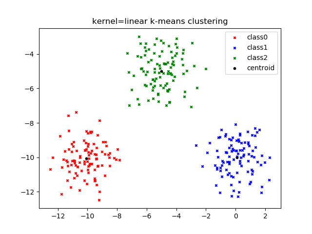
K-meansで分類できるデータセットは次のように各クラスで固まっている必要があります。

カーネルK-meansはK-meansの弱点を補います。
カーネルトリック
初めに、カーネルトリックを説明します。
線形分離できないようなデータ$X$を例えば次のように線形分離できるように$\phi(x)$に送る写像$\phi$を考えます。

カーネルは次のように定義されます。
$$K(x,y) = \phi(x)^T \phi(y)$$
$\phi$を具体的に計算することは難しいですが、$K(x,y)$を計算することなら簡単です。
この手法をカーネルトリックと呼ばれます。
カーネルK means
K-meansの目的関数を復習しておきます。
$$J = \sum_{n=1}^{N} \sum_{k=1}^{K} r_{nk} ||x_n-\mu_k||^2$$
ここで、 プロトタイプは$\mu_i ~\forall k \in K$とします。
$r_n$は1 of K符号化法であり、$r_{nk}$は$r_n$のk番目の要素です。
この時、
$$\mu_k = \frac{\sum_{n} r_{n_k} x_n}{\sum_n r_{n_k}}$$
そして、
$$k = \arg \min_{j} || x_n - \mu_{j} || \implies r_{nk} = 1$$
$$else \implies r_{n_k} = 0$$
次のように目的関数を書き換えます。
$$J = \sum_{n=1}^{N} \sum_{k=1}^{K} r_{nk} ||\phi(x_n)-\mu_k||^2$$
その時、
$$\mu_k = \frac{\sum_{n} r_{n_k} \phi(x_n)}{\sum_n r_{n_k}}$$
それゆえ、$x_n$とプロトタイプ$\mu_k$の距離は
$$||\phi(x_n) - \frac{\sum_{m}^{N} r_{m_k} \phi(x_m)} {\sum_{m}^{N} r_{m_k}} ||^2$$
$$= \phi(x_n)^T \phi(x_n) - \frac{2 \sum_{m}^{N} r_{n_k} \phi(x_n)^T \phi(x_m)}{\sum_{m}^{N} r_{n_k}} + \frac{\sum_{m,l}^{N} r_{n_k} r_{n_k} \phi(x_m)^T \phi(x_l)}{ \{ \sum_{m}^{N} r_{n_k} \}^2 }$$
カーネルK-meansでは$\phi(x_n)^T \phi(x_m)$を$K(x_n,x_m)$として計算します。
Algorithm
Reference
カーネルK-meansの実装編も併せてご覧ください。
概要
- K-meansの弱点
- カーネルトリック
- カーネルK-means
- アルゴリズム
K-meansの弱点
例えば、次のようなデータを用意します。

このデータはK-meansによってうまく分類することはできません。なぜなら通常のK-meansでは、データとプロトタイプのユークリッド距離に依存しているからです。そのため、このような円状に分布しているデータはうまく分類することができません。 プロトタイプとはそれぞれのクラスにあり、そのクラスを代表するようなもののことです。K-meansでは各クラスの平均ベクトルとなります。それゆえ、以下のような分類になってしまいます。

このようなデータではK-meansはうまくいきません。
K-meansで分類できるデータセットは次のように各クラスで固まっている必要があります。
カーネルK-meansはK-meansの弱点を補います。
カーネルトリック
初めに、カーネルトリックを説明します。
線形分離できないようなデータ$X$を例えば次のように線形分離できるように$\phi(x)$に送る写像$\phi$を考えます。

カーネルは次のように定義されます。
$$K(x,y) = \phi(x)^T \phi(y)$$
$\phi$を具体的に計算することは難しいですが、$K(x,y)$を計算することなら簡単です。
この手法をカーネルトリックと呼ばれます。
カーネルK means
K-meansの目的関数を復習しておきます。
$$J = \sum_{n=1}^{N} \sum_{k=1}^{K} r_{nk} ||x_n-\mu_k||^2$$
ここで、 プロトタイプは$\mu_i ~\forall k \in K$とします。
$r_n$は1 of K符号化法であり、$r_{nk}$は$r_n$のk番目の要素です。
この時、
$$\mu_k = \frac{\sum_{n} r_{n_k} x_n}{\sum_n r_{n_k}}$$
そして、
$$k = \arg \min_{j} || x_n - \mu_{j} || \implies r_{nk} = 1$$
$$else \implies r_{n_k} = 0$$
次のように目的関数を書き換えます。
$$J = \sum_{n=1}^{N} \sum_{k=1}^{K} r_{nk} ||\phi(x_n)-\mu_k||^2$$
その時、
$$\mu_k = \frac{\sum_{n} r_{n_k} \phi(x_n)}{\sum_n r_{n_k}}$$
それゆえ、$x_n$とプロトタイプ$\mu_k$の距離は
$$||\phi(x_n) - \frac{\sum_{m}^{N} r_{m_k} \phi(x_m)} {\sum_{m}^{N} r_{m_k}} ||^2$$
$$= \phi(x_n)^T \phi(x_n) - \frac{2 \sum_{m}^{N} r_{n_k} \phi(x_n)^T \phi(x_m)}{\sum_{m}^{N} r_{n_k}} + \frac{\sum_{m,l}^{N} r_{n_k} r_{n_k} \phi(x_m)^T \phi(x_l)}{ \{ \sum_{m}^{N} r_{n_k} \}^2 }$$
カーネルK-meansでは$\phi(x_n)^T \phi(x_m)$を$K(x_n,x_m)$として計算します。
Algorithm
- プロトタイプの初期値、K:クラスの数
- for iteration in iteration times.
- for $n \in N$ do
- for $k \in K$ do
- $x_n$とクラスkのプロトタイプの距離を計算します。
- end for k
- $x_n$とクラスkのプロトタイプの距離の中で最小にさせるようなクラス$k_n$を選びます。
- $x_n$のクラスを$k_n$とします。
- end for n
- もし、プロトタイプベクトルにほとんど変化がない場合はカーネルK-meansを終了します。
Reference
コメント
コメントを投稿